Statistics for the Working Mathematician

I’m a mathematician, but I managed to avoid almost all education about statistics, and I have found that statistics resources are often catered to a non-mathematician audience. So, to crystalize my own understanding (and in case it helps someone else), I wanted to write up a short introduction to statistics, focusing on “what do they do and why”, written to assume a familiarity with math (calculus and perhaps some measure theory).
Probability vs Statistics
Crudely speaking, probability and statistics are inverse problems. In probability, you are given a description of a world, and want to calculate the chance of an event happening. In statistics, you are given an event that happened (or N events) and wish to make a description of the world.
The descriptions of the world can be both qualitative and quantitative. For instance, statistics can be used to ask “does any binomial distribution fit this data?” or “knowing this a binomial distribution, what value(s) of the p parameter are most likely?”
Statistics in Seven Steps
Here’s how a basic problem in statistics might go. Throughout, we’ll use the example of determining if a coin is fair.
You have a hypothesis you want to test, and design a test that will let you separate your hypothesis from relevant alternatives.
In our example, we’ll take the hypothesis “the coin is fair”. If we say the chance of the coin coming up heads is θ, then we’re asking if θ=50%. Our test will be to flip the coin 100 times, and counting the number of heads.
You make (good or bad) assumptions about the process that produced the data.
In our example, we assume the coin’s probability θ is the same between flips, that the flips are independent, etc.
Using probability theory (or looking it up in a book), you create a family of probability density functions P_θ(x) based on your assumptions, with a parameter θ1, describing the chance of outcome x.
In our example, P_θ(x) is the binomial distribution (interactive) - the probability of flipping x heads if the coin comes up heads with probability θ.
You take some measurement x=S.
In our example, lets say 60 coin flips come up heads, so S=60.
Unfortunately, S might be such a small part of your space of x’s that P_θ(S) might be nearly 0, regardless of the choice of θ! How do we proceed?
It is a straightforward Calc 1 problem to show that if you fix x=60, the function P_θ(x)=(100 choose x) * θ^x * (1-θ)^(100-x) is maximized at θ=0.6, where P_{.6}(60)≈0.08. In other words, no matter how our coin is weighted, we’ll never have more than an 8% chance of flipping exactly 60 heads! We can also calculate that if the coin is fair, P_{.5}(60)≈0.01.
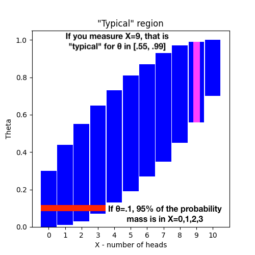
What we do instead is say S is a "typical" result (my term) for θ if S is in the middle 95% of the probability density function P_θ(x). That is, for each θ, we order all of the results you’d expect from P_θ(x), sorted by x, and take cutoffs at the 2.5th and 97.5th percentiles, resulting in some x cutoffs a(θ) and b(θ). Then x=S is typical if a(θ)<S<b(θ). Formally, a(θ) and b(θ) are the unique numbers satisfying the equations:

The confidence interval is the set of θ for which S is typical.
As described, we’d be using the Clopper-Pearson method2 to get our confidence interval, and an online calculator tells us our confidence interval is [0.4972, 0.6967], so a fair 50/50 coin is just barely within the interval, and we can say “our experiment does not rule out the possibility that the coin is fair”.

Let’s visualize the “typical” region for 10 coin flips:
Common Variants: p-values and one-sided tests
We made two arbitrary choices above, which we can address here:
Why do we choose the middle of the distribution? A common alternative is to look at the top or bottom 95% instead. Looking at the middle is called a two-tailed test since it excludes two extremal parts of the distribution, whereas looking at the top or bottom is called a one-tailed test. Each has their place, depending on the hypothesis you’re testing3.
In step 5, where did 95% come from? The choice was arbitrary, but industry standard. More generally, you can pick a significance threshold α (like 0.05), and test whether S is in the middle (1-α) of the distribution, which tells you whether or not your result is “statistically significant”.
The smallest α for which the result is in the middle (1-α) of the distribution is the p-value. So my understanding of the p-value is that it’s the probability that the result is a fluke even if all of your assumptions are right. But critically, the p-value does not say anything about:
Whether your assumptions were right
What would happen under alternative assumptions
Causality
Thus, the p-value is a lower bound on your result being wrong, in particular measuring the failure mode of “it happened by chance even though your assumptions were right”.
Point Estimates are Not Enough
But why bother with confidence intervals? Why can’t we just say our best guess at the possibility of the coin being fair?
This is of course a valuable thing to do, and it is called a point estimate! The technique of finding θ*=argmax_{θ} P(S,θ) is called maximum likelihood estimation, and is widely used.
But giving a point estimate can be insufficient to answer many statistical questions. Consider three coin-flipping experiments, with results:
6/10 flips are heads
60/100 flips are heads
6 million/10 million flips are heads
In all of these, the maximum likelihood estimate for θ is 0.6. But the implications for the hypothesis “our coin is fair” are very different:
In case (1), even with a fair coin there’s a 20% chance of getting 6/10 flips as heads, so this result is entirely consistent with a fair coin.
In case (2), the probability that a fair coin could only achieve ≥60/100 flips heads is only ~3%, so this is not the most common outcome, but still possible.
In case (3), its vanishingly unlikely that a fair coin could produce this result. You can say with near certainty that the coin is not fair.
A Bayesian Approach
We saw that 60/100 coins leaves the possibility of θ=.5 just barely within the confidence window. Suppose we instead get 61/100 heads, so θ=.5 is just outside the confidence window. Would you just to conclude the coin is unfair? Consider that we’ve interacted with thousands of coins in our lives, and they’ve almost always been fair. So consider two possibilities:
We picked up a completely normal coin and got slightly lucky in our flips.
We picked up a super-rare weighted coin and got a completely normal result in our flips.
Ignoring the common factor of “completely normal”, we can then compare being slightly lucky with case (1)’s flips to being extremely lucky with getting case (2)’s coin. Once we consider the rareness of weighted coins, we should realize that situation (1) is more plausible, even if it required getting some lucky flips.
This is of course Bayesian statistics. We combine our prior (almost all coins are fair) with our evidence (slight evidence of being unfair) to reach a posterior (this coin is probably fair). The exact mathematics of how to combine these numbers is Bayes’ law. Bayes’ law is very popular in some circles, and it holds out the possibility for being completely right about the entire state of the world.
However, I would raise two objections (which are hardly original to me):
While Bayes’ law describes how to update your prior, it is silent on how to make your prior, even though this step is equally essential to the process.
In our example, we know that weighted coins are rare, but how rare? One in one thousand? One in one million? To get an exact prior you must also include all other world information which might influence the odds of this coin being fair - does it look fake? Was it given to you by a stage magician? Has there been a recent rash of forgeries in the news? You can try to account for all these with Bayes’ law too, but they all ultimately need to draw from made-up priors. In some circumstances your conclusions are robust to a wide range of priors, and in some circumstances they are not.
You must track the entire probability distribution to properly apply Bayes’s law, which can get significant.
For instance, our coin may not be just “fair” or “unfair”, because not all unfair coins are the same. Instead you should track your entire probability distribution over θ in [0,1], so you’d need a computer to do any serious calculation.
Objections (1) and (2) combine to suggest that Bayesian statistics is at its most useful in cases where there are a relatively small number of possibilities, and your prior can be well-justified (for instance a game of chance with well-defined probabilities).
Parameters can be a single real value, as with θ, or can be vector-valued, or anything else.
Since binomial distributions are so common, and approximate normal distributions for large N and mid-size θ, there are a lot of other tests that approximate the confidence interval.
To be fully general, you could do statistics by defining any subset of frequency 95% as “typical”, even weird ones like “everything except the middle 5%”, or “the number of heads is not a perfect square” (if those probabilities worked out to 95%). But using order comparisons is nearly universal, for reasons I’ll speculate about here:
It’s easy, fast, and intuitive to compare number by ordering.
Order results respect linear operations such as averaging or rescaling.
By putting the cutoff in the tails (which are low probability), you minimize the boundary between “typical” and “atypical”, reducing the expected impact of noisy measurements.
By making your regions intervals, you only need to do a single integral/sum, and typically end up with nicer formulae than summing or integrating over weird sets.
There’s a well-defined order of “how atypical is this S”, allowing you to compute p-values.
Saying the extremes are atypical might be “better” at distinguishing between different distributions, which is a common concern. For instance, if D is a normal distribution with mean µ and standard deviation 1, and we’re testing the hypothesis that it’s a normal distribution with mean µ_0 and standard deviation 1, then the chance of a random draw S from D being in the “atypical” region is an increasing function of |µ-µ_0|. In contrast, if we say that the “atypical region” is the center 5% of a distribution, then the odds of S being in this atypical reason would actually go to 0 as |µ-µ_0| increases.
It’s good to have a standard to avoid p-hacking. Every result must lie in some percentile, so if you already know your result you could define your “typical” region to exclude your measurement. Thus order comparison serves serves as a form of pre-registration.